Looking at the most common flights per country in Asia

JY

Data Analyst, Ronin.

Looking at the most common flights per country in Asia

DataScience

Sep 4, 2021

I just wanted to see what were the main flights in Asian countries, following a viz I saw of the same for Europe.

Opensky published their “Crowdsourced air traffic data from the OpenSky Network 2019–2021” and I will only use the 2019 data, to focus on the situation before the pandemic.

2 IACO codes

Both origin and destination fields of the data use a 4-letter code which correspond to IACO codes. It makes data cleaning easier as, as opposed to IATA codes based on the airport name, IACO codes are based on the country/region the airport is located in.

My first approach was to refer to the map below to select the correct country codes, but I then went through Wikipedia pages on the topic and just extracted all airports 4-letter codes, instead of focusing on the 2 first characters.

IACO codes

    asia_iaco <- read_csv("iaco_asia.csv", col_types = "cf") %>%
      mutate(
        country = str_replace(country, "Hong Kong", "China"), ## Because rnaturalearth doesn't recognise HK
        country = str_replace(country, "Macau", "China"), ## Nor Macau
      )

    head(asia_iaco)

iaco	country
RCAY	Taiwan
RCBS	Taiwan
RCCM	Taiwan
RCDI	Taiwan
RCFG	Taiwan

3 Data loading

The complete worldwide dataset for 2019 is 2.3 GB. Compressed.

Dataset full size: 5.75GB

    opensky <- list.files("./raw_data/", pattern = "*.csv", all.files = TRUE, full.names = TRUE)

    flights <- opensky %>% 
      lapply(read_csv, col_types = "cccccccTTDdddddd") %>% 
      bind_rows()

    flights %>% head() %>% print()

#	callsign	icao24	registration	typecode	origin	destination

1	HVN19	888152			YMML	LFPG
2	CCA839	780ad1			YMML	LEBL
3	CES219	780b7e	B-5936	A332	YSSY	EDDF
4	AEA040	34444e	EC-LVL	A332	LEMD	LEMD
5	CXA825	780d75	B-2760	B788	YSSY	LFPG
6	TGW700	76bcca	9V-OFJ	B788		RJBB

## # … with 9 more variables: firstseen <dttm>, lastseen <dttm>, day <date>,
## #   latitude_1 <dbl>, longitude_1 <dbl>, altitude_1 <dbl>, latitude_2 <dbl>,
## #   longitude_2 <dbl>, altitude_2 <dbl>

    print(glue::glue("The total dataset contains {prettyNum(dim(flights)[1],big.mark=',',scientific=FALSE)} observations!"))

    ## The total dataset contains 30,989,481 observations!

This does take a long time to load but includes a lot of observations we are not interested in. Let’s clean that

    flights %>% 
      filter(
        origin %in% asia_iaco$iaco,
        destination %in% asia_iaco$iaco,
        origin != destination
      ) %>%
      left_join(asia_iaco, by = c("origin" = "iaco")) %>%
      left_join(asia_iaco, by = c("destination" = "iaco")) %>% 
      rename(
        country_origin = country.x,
        country_destination = country.y
      )-> asia_flights

    head(asia_flights) %>% knitr::kable(format = "pipe")

callsign	number	icao24	registration	typecode	origin	destination	firstseen	lastseen	day	latitude_1	longitude_1	altitude_1	latitude_2	longitude_2	altitude_2	country_origin	country_destination
SVA872	NA	710058	HZ-AK16	B77W	WIII	RPLL	2018-12-31 04:00:49	2019-01-01 05:54:59	NA	-6.123714	106.63216	0.0	14.49194	120.98954	99.06	Indonesia	Philippines
IGO2134	NA	800d34	NA	NA	VOBL	VOMM	2018-12-31 14:59:40	2019-01-01 00:55:29	NA	13.206218	77.72750	914.4	12.98547	80.15649	-38.10	India	India
IGO748	NA	800c97	NA	NA	VOMM	VABB	2018-12-31 15:02:13	2019-01-01 05:50:15	NA	12.982907	80.15914	-304.8	19.08842	72.84889	-22.86	India	India
JSA761	NA	76aa6b	9V-JSK	A320	WMKK	RPLL	2018-12-31 15:17:09	2019-01-01 01:59:12	NA	2.742532	101.67454	0.0	14.49335	120.99196	45.72	Malaysia	Philippines
UAL151	NA	a9d5e7	N73278	B738	RPLL	RJBB	2018-12-31 15:57:43	2019-01-01 00:45:55	NA	14.519440	121.03908	0.0	34.42145	135.19557	-68.58	Philippines	Japan
IGO872	NA	800716	VT-IFA	A320	VIDP	VOMM	2018-12-31 17:11:23	2019-01-01 00:13:45	NA	28.568270	77.07949	304.8	12.98184	80.14671	22.86	India	India

This gives us almost what we want. One qui modification will be to group flights by routes rather than by origin-destination pair. A Tokyo-Fukuoka flight should be grouped with its counterpart.

    asia_flights %>% 
      mutate(
        route = if_else(origin <= destination, paste0(origin, destination), paste0(destination, origin))
      ) %>% 
      group_by(country_origin, country_destination, route) %>%
      summarise(
        counter = n(),
        longitude_origin = median(longitude_1, na.rm = TRUE),
        latitude_origin = median(latitude_1, na.rm = TRUE),
        longitude_destination = median(longitude_2, na.rm = TRUE),
        latitude_destination = median(latitude_2, na.rm = TRUE),
      ) -> asia_flights_summary

    asia_flights_summary %>% head() %>% knitr::kable(format = "pipe")

country_origin	country_destination	route	counter	longitude_origin	latitude_origin	longitude_destination	latitude_destination
China	China	VHHHVHSK	829	113.9129	22.29801	114.1494	22.29666
China	China	VHHHVMMC	196	113.9098	22.30003	113.6387	22.15329
China	China	VHHHZBAA	27	113.9374	22.30907	116.5634	39.86545
China	China	VHHHZBHD	1	114.4551	36.54492	113.8526	22.29630
China	China	VHHHZBNY	6	113.9245	22.30476	116.6393	39.85443
China	China	VHHHZGGG	37	113.9208	22.30508	113.3811	23.16518

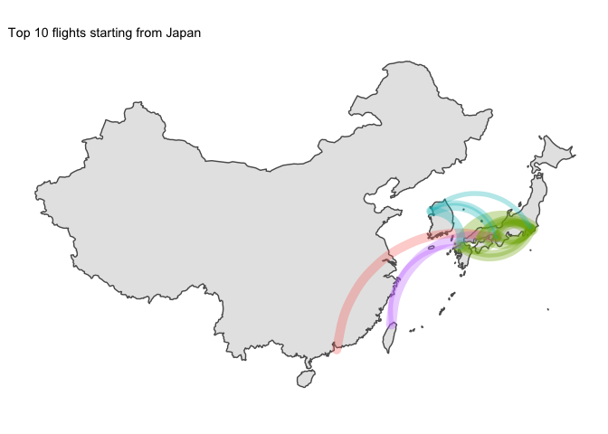
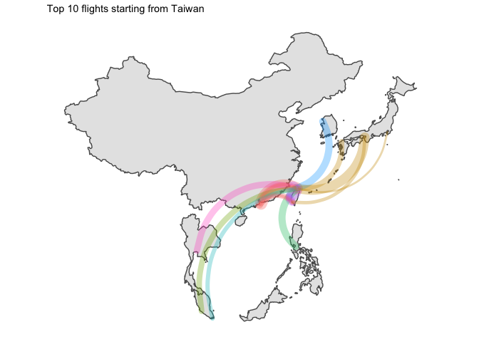
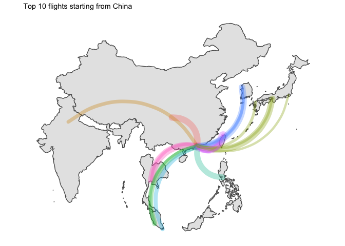
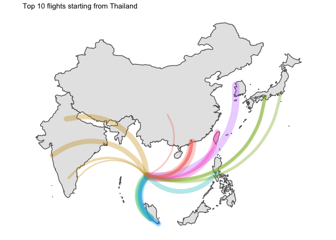
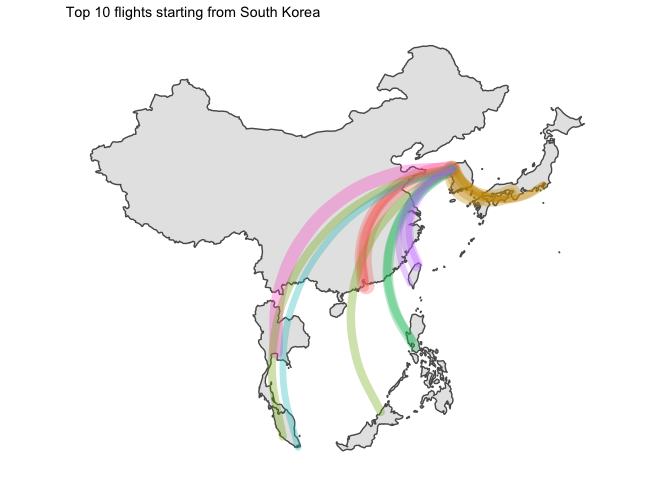
4 Time for a rough viz

Let’s have a first look at the graphs

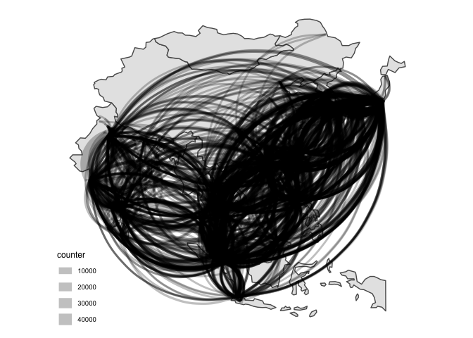
We’d better split that by country of origin.

    asia_flights_summary %>% 
      filter(longitude_origin > 0) %>% 
      arrange(desc(counter)) %>%
      group_by(country_origin) %>%
      mutate(ranking = row_number()) %>%
      ungroup() %>% 
      filter(ranking <= 10) -> graph_ready_data

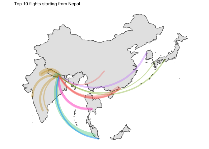
    for (ctry in unique(graph_ready_data$country_origin)){
      g <- graph_ready_data %>%
        filter(country_origin == ctry) %>%
        ggplot() +
        geom_sf(data = ne_countries(country = ctry, returnclass = "sf", scale = "medium")) +
        geom_curve(
          aes(
            x = longitude_origin, xend = longitude_destination, 
            y = latitude_origin, yend = latitude_destination,
            size = counter, colour = 
            ),
          lineend = "round"
          ) +
        theme_map() +
        labs(
          title = glue::glue("Top 10 flights starting from {ctry}")
        ) + 
        theme(
          legend.position = "none"
        )
      
      print(g)
    }

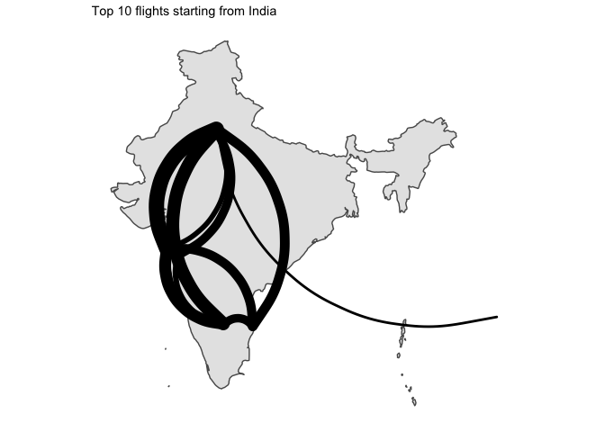
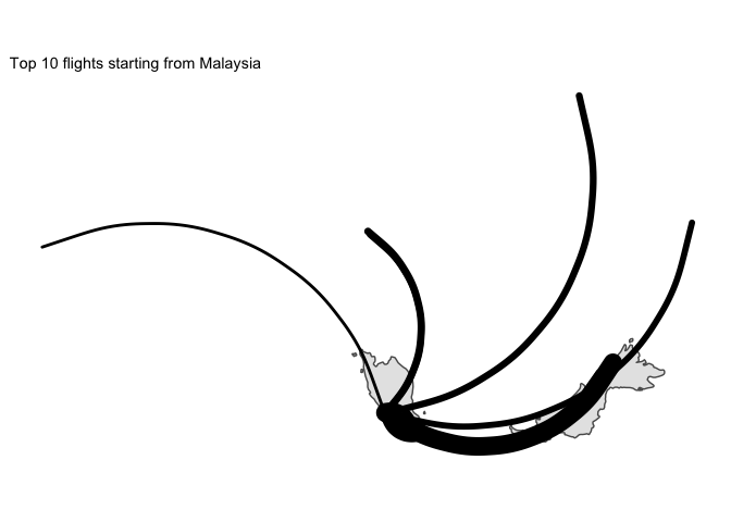
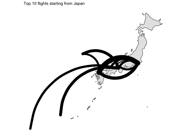
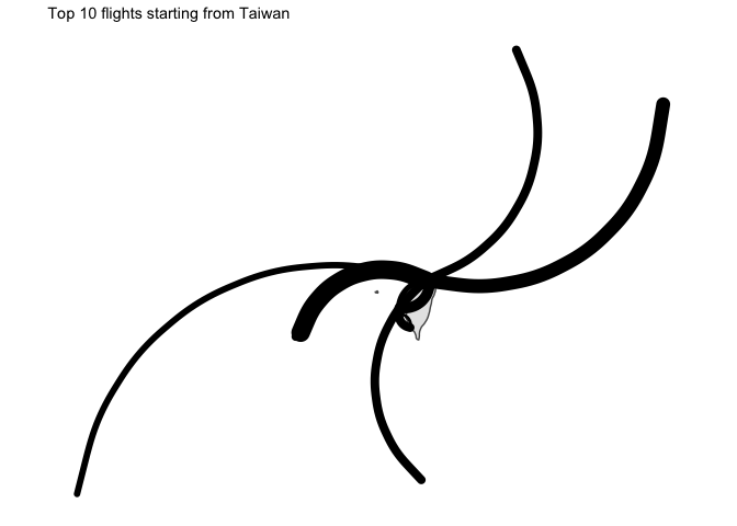
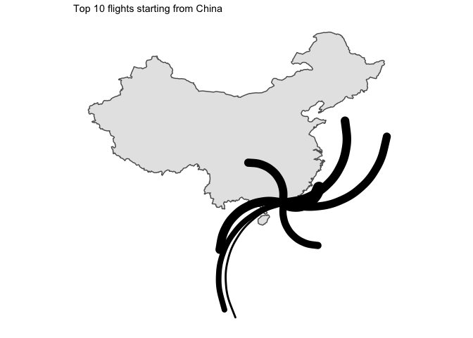
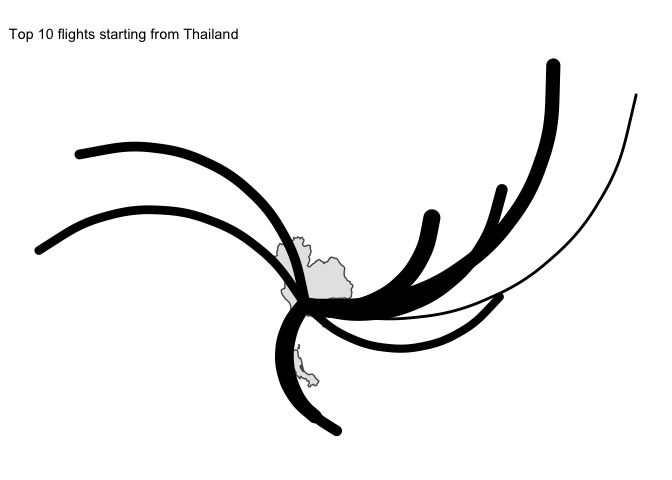
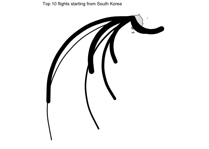
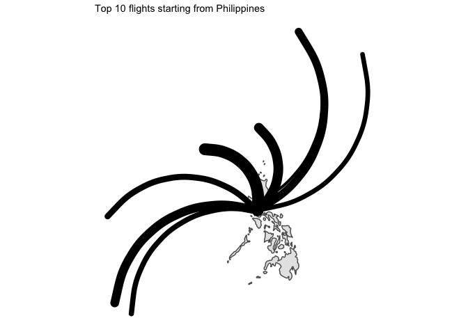
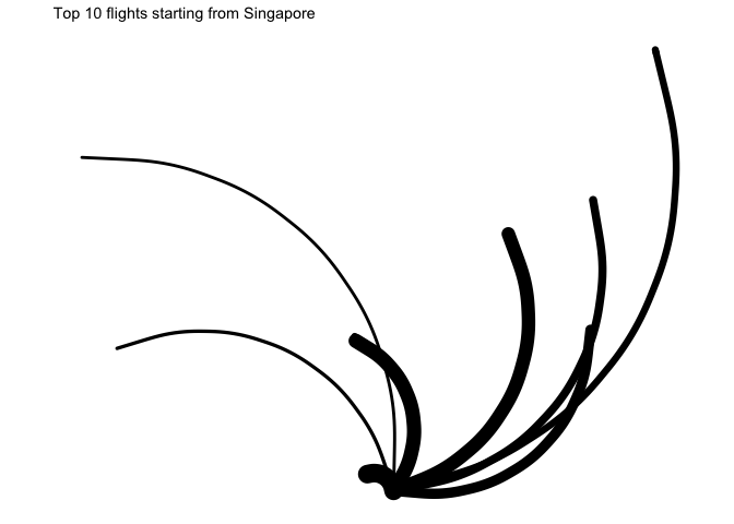
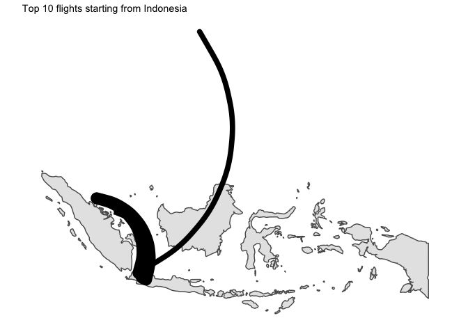
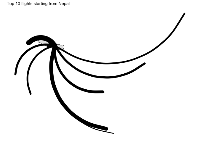
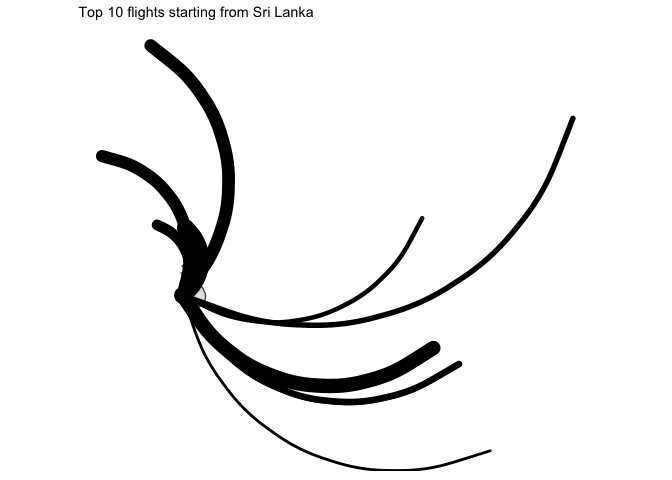
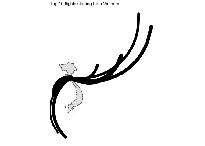
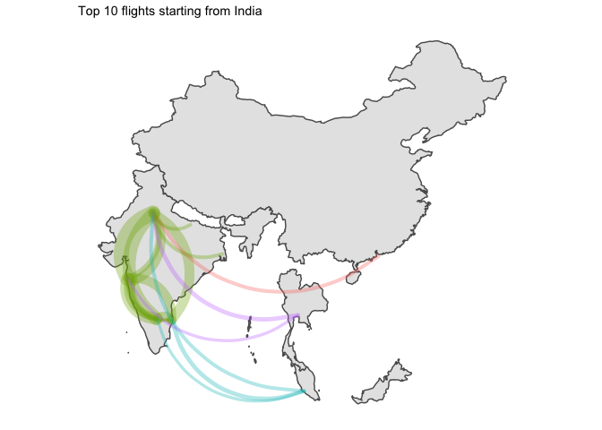
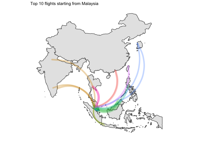
I… kind of like the way it looks ? But without seeing the destination country, that is not that useful.

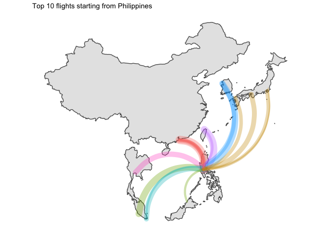
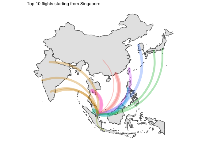
asia_flights_summary %>% 
  filter(longitude_origin > 0) %>% 
  arrange(desc(counter)) %>%
  group_by(country_origin) %>%
  mutate(ranking = row_number()) %>%
  ungroup() %>% 
  filter(ranking <= 20) -> graph_ready_data

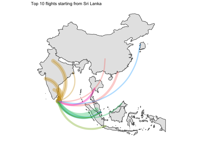
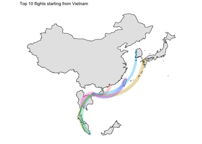
for (ctry in unique(graph_ready_data$country_origin)){
  all_ctry <- graph_ready_data %>% filter(country_origin == ctry) %>% select(country_destination) %>% unique() %>% pull(country_destination)
  g <- graph_ready_data %>%
    filter(country_origin == ctry) %>%
    ggplot() +
    geom_sf(data = ne_countries(country = all_ctry, returnclass = "sf", scale = "medium")) +
    geom_curve(
      aes(
        x = longitude_origin, xend = longitude_destination, 
        y = latitude_origin, yend = latitude_destination,
        size = counter, colour = country_destination
        ),
      lineend = "round", alpha = 0.33
      ) +
    theme_map() +
    labs(
      title = glue::glue("Top 10 flights starting from {ctry}")
    ) + 
    theme(
      legend.position = "none"
    )
  
  print(g)
}

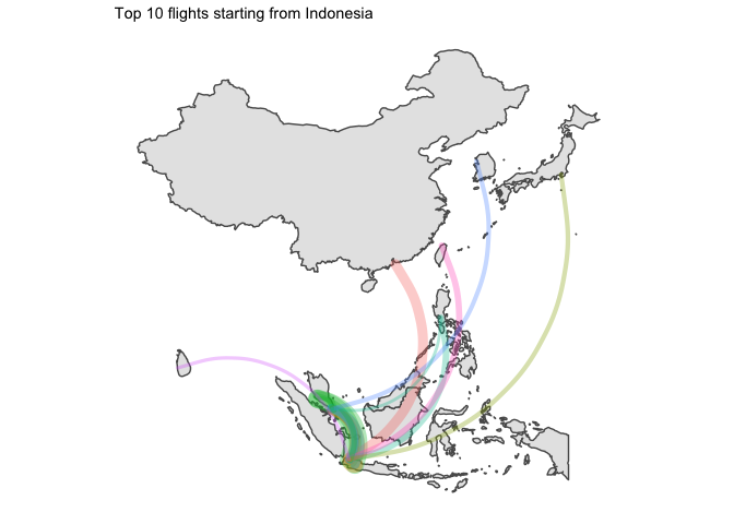
5 Final word

Not much to say. This was a quick and dirty data playground to take my mind off of life.

Two points of interest:

Japan was the only country which had domestic flights in its top 10 routes
I am disappointed by the lack of data for China. Only available flights are for HK which leaves most of the country blank…