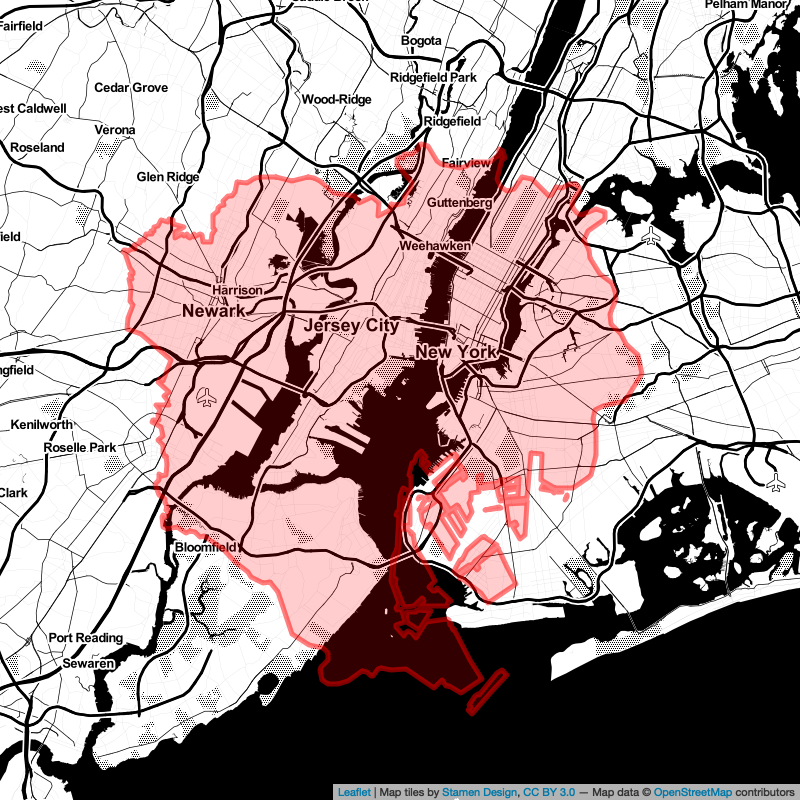
I have finally had the time to dive into spatial data correctly, partially because my new job has a strong spatial element to it. This revived a side project I had put aside for a few months: comparing the size of Tokyo with other major cities.
Code:
library(tidyverse)
library(sf)
library(leaflet)
library(htmlwidgets)
library(webshot)


tokyo <- st_read("./shapefiles/japan_cities.shp") %>%
  filter(
    KEN == "東京都",
    str_detect(SIKUCHOSON, "区")
  ) %>%
  st_make_valid() %>%
  st_union() %>%
  st_transform(crs = 4326) %>%
  st_as_sf()

paris <- c(2.34682, 48.85522) # Cité
london <- c(-0.12536, 51.50090) # Big Ben
ny <- c(-74.04455, 40.68917) # Statue of liberty
pekin <- c(116.39703, 39.91346) # Forbidden City

lets_move_to <- function(target, output_suffix = NA){
    zoom = 11

    # adjusting the position of the tokyo object so that the center/centroid matches with the Imperial Palace
    kokyo_adjustment <- st_centroid(tokyo)%>% st_coordinates() %>% as_vector() - c(139.75272, 35.68488)

    tokyo_moved <- tokyo

    ## Here is where the translation is done
    st_geometry(tokyo_moved) <- (
            st_geometry(tokyo_moved) -
            st_centroid(tokyo)%>% st_coordinates() %>% as_vector() +
            kokyo_adjustment +
            target)

    st_crs(tokyo_moved) <- st_crs(tokyo)

    m <- leaflet(tokyo_moved) %>%
    addTiles() %>%
    addPolygons(fillColor = "red", color = "red", stroke = 1)

    if(!is.na(output_suffix)){
    fname = paste("./out/tokyo_to_",output_suffix,".png", sep = "_")
    } else
    {
    fname = "./out/map_output.png"
    }

    saveWidget(m, "./tmp/temp.html", selfcontained = FALSE)
    webshot("./tmptemp.html", file = fname,
            cliprect = "viewport",
            vwidth = 800,
            vheight = 800)
    m
}

lets_move_to(paris, "paris")
lets_move_to(london, "london")
lets_move_to(pekin, "pekin")
lets_move_to(ny, "ny")
outputs
Discussion
General
Working with {sf} in itself was great. No issue there. I just needed to get used to the API but the main difficulty was to align what I had in mind with the data I could find. And get used to working with different CRS. That last point is far from being clear for me now.
Translation
That piece of code is where the actual translation is done.
st_geometry(tokyo_moved) <- (
        st_geometry(tokyo_moved) -
        st_centroid(tokyo)%>% st_coordinates() %>% as_vector() +
        target +
        kokyo_adjustment)
The only slight adjustment I had to do was to add this kokyo_adjustment variable. As useful as the polygon centroid (in green below) is, it does not correspond with what is usually regarded as the geographical center of Tokyo: the Imperial Palace (in red). What counts as the center of Tokyo could be lead to endless discussions, Wikipedia lists it as the Prefectural government. Others would consider Tokyo Station, others Shinjuku.
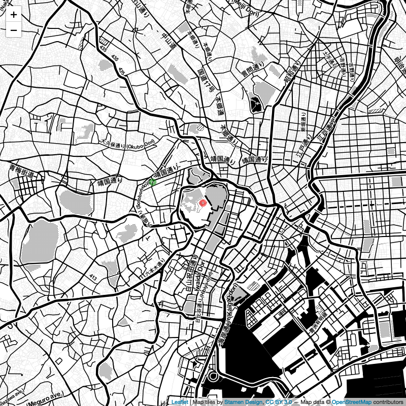
In the same way, all the target coordinates I have listed correspond to landmarks in the targets cities rather than a mathematically accurate-ish center.
Saving a {leaflet} map
The final hurdle I had was how to save the output from the {leaflet} package. Thankfully, StackOverflow had the answer
saveWidget(m, "./tmp/temp.html", selfcontained = FALSE)
    webshot("./tmptemp.html", file = fname,
            cliprect = "viewport",
            vwidth = 800,
            vheight = 800)